Histfactory
HistFactory [^hf] is a language to describe statistical models consisting only of "histograms" (which is used interchangeably with "step-functions" in this context). Each HistFactory distribution describes one "channel" or "region" of a binned measurement, containing a stack of "samples", i. e. binned distributions sharing the same binning (step-functions describing the signal or background of a measurement). Such a HistFactory model is shown in Figure 1 (originally from [^atlashzz]). Each of the contributions may be subject to modifiers.
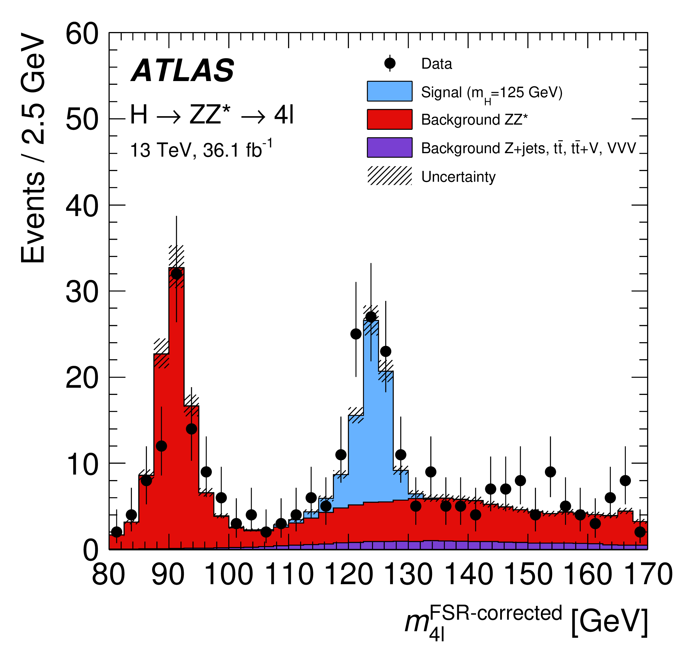
The prediction for a binned region is given as
Here \(d_s(x)\) is the prediction associated with the sample \(s\), a step function
In this section, \(\chi^{y_s}_{b}(x)\) denotes a generic step function in the binning \(b\) such that \(\chi_{b}(x) = y_{s,i}\), some constant, if \(x\in[b_i,b_{i+1})\). The \(y_{s,i}\) in this case are the bin contents (yields) of the histograms. The \(M_\kappa\) are the multiplicative modifiers, the \(M_\delta\) are the additive modifiers. Each of the modifiers is either multiplicative (\(\kappa\)) or additive (\(\delta\)). All samples and modifiers share the same binning \(b\). The modifiers depend on a set of nuisance parameters \(\theta\), where each modifier can only depend on one \(\theta_i\), but the \(\theta_i\) can take the form of vectors and the same \(\theta_i\) can be shared by several modifiers. By convention, these are denoted \(\alpha\) if they affect all bins in a correlated way, and \(\gamma\) if they affect only one bin at a time. The types of modifiers are
- A uncorrelated shape systematic or
shapefactormodifier is a multiplicative modifier that scales each single bin by the value of some independent parameter \(\gamma\). Here, \(\theta_i=\vec{\gamma}\), where the length of \(\vec{\gamma}\) is equal to the number of bins in this region. This type of modifier is sometimes calledshapesys, with some nuance in the meaning. However, both are synonymous in the context of this standard. - A correlated shape systematic or
histosysmodifier is an additive modifier that adds or subtracts a constant step function \(\chi^f\), scaled with a single factor \(\alpha\). The modifier contains adatasection, which contains the subsections \(\texttt{hi}\) and \(\texttt{lo}\) that help to define the step function \(\chi^f\). They containcontents, which define the bin-wise additions or subtractions for \(\alpha=1\). Here, \(\theta_i=\alpha\). - A normalization systematic or
normsysmodifier is a multiplicative modifier that scales the entire sample with the same constant factor \(f\) that is a function of \(\alpha\). The modifier contains adatasection, which contains the values \(\texttt{hi}\) and \(\texttt{lo}\) that help to define \(f\). There are different functional forms that can be chosen for \(f\). However, by convention \(f(\alpha=0)=1\), \(f(\alpha=+1)=\)"hi" and \(f(\alpha=-1)=\)"lo". In this case, \(\theta_i=\alpha\). - A normalization factor or
normfactormodifier is a multiplicative modifier that scales the entire sample in this region with the value of the parameter \(\mu\) itself. In this case, \(\theta_i=\mu\). - The
staterrormodifier is a shorthand for encoding uncorrelated statistical uncertainties on the values of the step-functions, using a variant1 of the Barlow-Beeston Method [^barlowbeeston]. Here, the relative uncertainty on the sum of all samples in this region containing thestaterrormodifier is computed bin-by-bin. Then, a constrained uncorrelated shape systematic (shapesys) is created, encoding these relative uncertainties in the correspondingPoisson(orGaussian) constraint term.
The different modifies and their descriptions are also summarized in the following table:
| Type of Modifier | Description | Definition | Free Parameters | Number of Free Parameters |
|---|---|---|---|---|
histosys |
Correlated Shape systematic | \(\delta(x,\alpha) = \alpha * \chi_b^f\) | \(\alpha\) | 1 |
normsys |
Normalization systematic | \(\kappa(x,\alpha) = f(\alpha)\) | \(\alpha\) | 1 |
normfactor |
Normalization factor | \(\kappa(x,\mu) = \mu\) | \(\mu\) | 1 |
shapefactor, staterror |
Shape factor | \(\kappa(x,\vec{\gamma}) = \chi_b^{\gamma}\) | \(\gamma_0\), ..., \(\gamma_n\) | #bins |
The staterror modifier is a special subtype of shapefactor, where the mean of the constraint is given as the sum of the predictions of all the samples carrying a staterror modifier in this bin.
The way modifiers affect the yield in the corresponding bin is subject to an interpolation function. The overallsys and histosys modifiers thus allow for an additional key interpolation, which identifies one of the following functions:
lin: \(\begin{cases} y_{\mathrm{nominal}} + x \cdot (y_{\mathrm{high}} - y_{\mathrm{nominal}}) \text{ if } x\geq0\\ y_{\mathrm{nominal}} + x \cdot (y_{\mathrm{nominal}} - y_{\mathrm{low}}) \text{ if } x<0 \end{cases}\)log: \(\begin{cases} y_{\mathrm{nominal}} \cdot \left(\frac{y_{\mathrm{high}}}{y_{\mathrm{nominal}}}\right)^x \text{ if } x\geq0\\ y_{\mathrm{nominal}} \cdot \left(\frac{y_{\mathrm{low}}}{y_{\mathrm{nominal}}}\right)^{-x}\text{ if } x<0 \end{cases}\)parabolic: \(\begin{cases} y_{\mathrm{nominal}} + (2s+d)\cdot(x-1)+(y_{\mathrm{high}} - y_{\mathrm{nominal}}) \text{ if } x>1\\ y_{\mathrm{nominal}} - (2s-d)\cdot(x+1)+(y_{\mathrm{low}} - y_{\mathrm{nominal})}\text{ if } x<-1\\ s \cdot x^2 + d\cdot x \text{ otherwise} \end{cases}\) with \(s=\frac{1}{2}(y_{\mathrm{high}} + y_{\mathrm{low}}) - y_{\mathrm{nominal}}\) and \(d=\frac{1}{2}(y_{\mathrm{high}} - y_{\mathrm{low}})\)poly6: \(\begin{cases} y_{\mathrm{nominal}} + x \cdot (y_{\mathrm{high}} - y_{\mathrm{nominal}}) \text{ if } x>1\\ y_{\mathrm{nominal}} + x \cdot (y_{\mathrm{nominal}} - y_{\mathrm{low}}) \text{ if } x<-1\\ y_{\mathrm{nominal}} + x \cdot (S + x \cdot A \cdot (15 + x^2 \cdot (3x^2-10))) \text{ otherwise} \end{cases}\) with \(S = \frac{1}{2}(y_{\mathrm{high}} - y_{\mathrm{low}})\) and \(A=\frac{1}{16}(y_{\mathrm{high}} + y_{\mathrm{low}} - 2\cdot y_{\mathrm{nominal}})\)
Modifiers can be constrained. This is indicated by the component constraint, which identifies the type of the constraint term. In essence, the likelihood picks up a penalty term for changing the corresponding parameter too far away from its nominal value. The nominal value is, by convention, defined by the type of constraint, and is 0 for all modifiers of type sys (histosys, normsys) and is 1 for all modifiers of type factor (normfactor, shapefactor). The strength of the constraint is always such that the standard deviation of constraint distribution is \(1\).
The supported constraint distributions, also called constraint types, are Gauss for a gaussian with unit width (a gaussian distribution with a variance of \(1\)), Poisson for a unit Poissonian (e.g. a continous Poissonian with a central value 1), or LogNormal for a unit LogNormal,. If a constraint is given, a corresponding distribution will be considered in addition to the aux_likelihood section of the likelihood, constraining the parameter to its nominal value.
An exception to this is provided by the staterror modifier as described above, and the shapesys for which a Poissonian constraint is defined with the central values defined as the squares of the values defined in vals.
The components of a HistFactory distribution are:
name: custom unique stringtype:histfactory_distaxes: array of structs representing the axes. If given each struct needs to have the componentname. Further, (optional) components aremax,minandnbins, or, alternatively,edges. The definition of the axes follows the format for binned data (see Section Binned Data).samples: array of structs containing the samples of this channel. For details see below. Struct of one sample:name: (optional) custom string, unique within this functiondata: struct containing the componentscontentsanderrors, depicting the data contents and their errors. Both components are arrays of the same length.modifiers: array of structs with each struct containing a componenttypeof the modifier, as well as a componentparameter(defining a string) or a componentparameters(defining an array of strings) relating to the name or names of parameters controlling this modifier. Further (optional) components aredataandconstraint, both depending on the type of modifier. For details on these components, see the description above. Two modifiers are correlated exactly if they share the same parameters as indicated byparameterorparameters. In such a case, it is mandatory that they share the same constraint term. If this is not the case, the behavior is undefined.
{
  "name": "myAnalysisChannel",
  "type": "histfactory_dist",
  "axes": [
    { "max": 1.0, "min": 0.0, "name": "myRegion", "nbins": 2 }
  ],
  "name":"myChannel1",
  "samples": [
    {
      "name": "mySignal",
      "data": { "contents": [ 0.5, 0.7 ], "errors": [ 0.1, 0.1 ] },
      "modifiers": [
        { "parameter": "Lumi", "type": "normfactor" },
        { "parameter": "mu_signal_strength", "type": "normfactor" },
        { "constraint": "Gauss", "data": { "hi": 1.1, "lo": 0.9 },
          "parameter": "my_normalization_systematic_1",
          "type": "normsys" },
        { "constraint": "Poisson", "type": "staterror",
          "parameters": ["gamma_stat_1","gamma_stat_2"]},
        { "constraint": "Gauss", "type": "histosys",
          "data": {
            "hi": { "contents": [ -2.5, -3.1 ] },
            "lo": { "contents": [ 2.2, 3.7 ] }
           },
           "parameter": "my_correlated_shape_systematic_1" },
        { "constraint": "Poisson", "data": { "vals": [ 0.0, 1.2 ] },
          "parameter": "my_uncorrelated_shape_systematic_2",
          "type": "shapesys" }
      ]
    },
    {
      "name": "myBackground",
      ...
   }
  ]
}
-
The variation consists of summarizing all contributions in the stack to a single contribution as far as treatment of the statistical uncertainties is concerned. ↩